Moment Energy
Full-Stack Software Engineer Co-op
Timespan
Jan 2025 - Aug 2025
Tools
React, MUI, NestJS, AWS (IoT Core, Athena, S3, SES), MySQL, Prisma
Overview
At Moment Energy, I built production software for monitoring battery energy storage systems (BESS systems), spanning React dashboards, NestJS services, and AWS telemetry infrastructure. My work helped reduce live telemetry API response times by approximately 70% and deliver a cloud fault detection system deployed to production with dashboard and email alerts.

The Moment Energy team. Source: Moment Energy
Core Contributions
Telemetry Dashboard Query Optimization
Impact: Live telemetry API response times fell by approximately 70%. Supported query ranges expanded from days to weeks, and long-running queries dropped from several minutes to seconds.
Problem: Querying historical battery telemetry became increasingly expensive as the requested time range grew. The legacy Express backend retrieved large volumes of sensor readings and performed additional aggregation and transformation in application code, resulting in extremely long API response times, limited practical query ranges due to http timeouts, and poor user experience.
As part of our architecture overhaul, I contributed to the Telemetry Service, which was originally part of the legacy Express monolithic backend. I diagnosed, then rebuilt the telemetry pipeline across Athena, the API, and the React dashboard, combining several layers of optimization:
SQL optimization: Athena/Presto SQL with CTEs, timestamp-based downsampling, window functions, and aggregation to process telemetry closer to its source.
Reduced backend computation: Moved BESS rack/module and cell-level calculations into Athena, reducing CPU-intensive processing on the EC2-hosted Node.js service.
Efficient data processing: Simplified API response construction and frontend data transformations, using map-based lookups where appropriate.
Response compression: Enabled Gzip in the NestJS API to reduce transfer sizes, particularly for larger telemetry responses.
Selective Downsampling Telemetry
Longer query ranges returned increasingly large telemetry datasets. I adjusted sampling resolution to the requested range, returning fewer readings while preserving a useful view of battery behavior. Our queries also filtered on partition keys so Athena could skip irrelevant S3 partitions.
Readings generally arrived every 10 seconds, but irregular timing, gaps, and restarts meant they did not always align with sampling targets. Rather than requiring exact matches, I grouped readings into time buckets and ranked each sensor’s readings by proximity to the target timestamp, selecting the closest available reading in each bucket.
The query followed these stages:
Read telemetry for the selected pack and time range
Assign each reading to a time bucket

For each sensor in each bucket:
    Keep the reading closest to the target timestamp

For each pack in each bucket:
    Calculate minimum and maximum voltage
    and maximum temperature across the selected readings

Return structured results for the dashboard
I organized these stages using Athena/Presto Common Table Expressions (WITH ... AS), separating filtering, bucketing, ranking, and aggregation into readable steps. This made the transformations easier to inspect and maintain while keeping the processing in Athena.
SQL example
Illustrative SQL, not production source: This example uses a simplified schema, one-minute buckets, and midpoint targets to demonstrate the approach. These intervals and targets do not represent confirmed production settings. Here, sensor_id identifies an independent measurement stream within a pack. Partition-key filters are omitted from this example.
WITH filtered AS (
    SELECT
        pack_id,
        sensor_id,
        reading_timestamp,
        cell_voltage,
        temperature
    FROM telemetry
    WHERE pack_id = 'example-pack'
      AND reading_timestamp >= TIMESTAMP '2025-01-01 00:00:00'
      AND reading_timestamp < TIMESTAMP '2025-01-01 01:00:00'
),
bucketed AS (
    SELECT
        *,
        date_trunc('minute', reading_timestamp) AS time_bucket
    FROM filtered
),
candidates AS (
    SELECT
        *,
        date_add('second', 30, time_bucket) AS target_timestamp
    FROM bucketed
),
ranked_telemetry AS (
    SELECT
        *,
        ROW_NUMBER() OVER (
            PARTITION BY pack_id, sensor_id, time_bucket
            ORDER BY ABS(
                date_diff(
                    'millisecond',
                    reading_timestamp,
                    target_timestamp
                )
            ), reading_timestamp
        ) AS timestamp_rank
    FROM candidates
)
SELECT
    pack_id,
    time_bucket,
    MIN(cell_voltage) AS min_cell_voltage,
    MAX(cell_voltage) AS max_cell_voltage,
    MAX(temperature) AS max_temperature
FROM ranked_telemetry
WHERE timestamp_rank = 1
GROUP BY pack_id, time_bucket
ORDER BY pack_id, time_bucket;
Each reading belongs to the minute containing its timestamp; only readings from that bucket compete for its midpoint target. Ranking by distance selects an actual reading even when arrivals are irregular. For example, readings at 12:00:26 and 12:00:41 compete for 12:00:30, and the former wins. A reading at 12:01:00 belongs to the next bucket. A bucket with no readings produces no sampled row.
The final aggregation calculates measurement extremes across the selected sensor readings in each bucket. It does not capture every extreme that occurred between those readings.
This approach reduced the number of records the backend and dashboard needed to process. However, selecting representative readings introduced a tradeoff: brief spikes or anomalies between those readings could be missed. Preserving those events became an additional stage of the optimization work (Detecting and Flagging Telemetry Anomalies).
Aggregating battery measurements
The dashboard needed summaries across battery racks, modules, and cells, including voltage extremes and maximum temperature. The legacy backend calculated these by iterating through query results, increasing processing work for longer queries.
I moved these calculations into Athena:
- Aggregation: Used
GROUP BYto organize readings by battery component and time interval, thenMIN()andMAX()to calculate measurement extremes. - Missing values: Used
COALESCE()where appropriate to handle missing measurement fields within the query.
The backend could then assemble responses from aggregated results, giving the dashboard data ready for visualization.
Streamlining the API and dashboard
Moving downsampling and aggregation into Athena reduced the work required in application code. I then focused on how the backend assembled the remaining results and how the dashboard consumed them.
In the NestJS response builder, I replaced repeated array scans with JavaScript Set and Map lookups, reducing redundant processing during response assembly. The React dashboard consumed the structured query results with fewer transformations before rendering charts.
Together, these changes simplified the path from stored telemetry to visualization:
| Stage | Before | After |
|---|---|---|
| Athena | Returned relatively raw readings | Filtered, downsampled, and aggregated readings |
| EC2-hosted backend | Grouped readings, calculated measurement extremes, and assembled responses | Assembled responses from structured results using Set and Map lookups |
| React dashboard | Performed additional chart transformations | Consumed data already shaped for visualization |
I also enabled Gzip compression for API responses, reducing the amount of data transferred to the dashboard, particularly for larger telemetry payloads.
The revised pipeline reduced synchronous processing on the Node.js backend, redundant transformations in React, and response transfer sizes. Alongside the query optimizations, these changes helped reduce API response times by approximately 70% and made longer time ranges practical to explore.
Detecting and Flagging Telemetry Anomalies
Battery telemetry could contain brief spikes or sudden shifts to a sustained higher or lower operating level. I needed to flag these anomalies as readings arrived and retain their timestamps for later investigation.
Fast detection without repeatedly querying large volumes of historical telemetry led me to explore online algorithms. These algorithms update compact running statistics with each incoming reading, allowing the detector to evaluate new measurements without retrieving or reprocessing the full history.
I used the live MQTT telemetry stream to track a running exponential moving average (EMA), identifying readings that departed significantly from a device/sensor's recent behavior. This could flag both short-lived anomalies and the onset of sustained changes, preserving the first detected reading's timestamp.
These flags also addressed a limitation of downsampling: readings selected five minutes apart might barely differ even though a sharp spike occurred between them. Reducing data for visualization could hide that event.
We stored the timestamps identified by the live anomaly detector. When a long-range query covered those timestamps, we included their readings alongside the downsampled data regardless of whether regular sampling would select them. This kept flagged events visible while reducing the overall chart payload.
Choosing the right baseline was important because it determined which readings were considered anomalous. It needed to represent a sensor's recent behavior as its normal operating level changed.
Alternatives explored: Welford and Chan
I explored Welford's running mean and variance for a running z-score, along with Chan's parallel variance formula. Both offered compact statistical summaries without retaining the full time-series history in detector memory.
Welford updates a count n, mean mean, and sum of squared deviations M2 for each new reading x:
n_new    = n + 1
delta    = x - mean
mean_new = mean + delta / n_new
M2_new   = M2 + delta * (x - mean_new)

sample_variance = M2_new / (n_new - 1)
Sample variance requires at least two readings. A new reading can be scored against the prior summary using z = (x - mean) / sqrt(sample_variance), with sufficient history and nonzero variance.
Chan's formula merges two summaries, A and B:
n     = n_A + n_B
delta = mean_B - mean_A
mean  = mean_A + delta * n_B / n
M2    = M2_A + M2_B + delta^2 * n_A * n_B / n
This lets you combine batches or partitions without replaying their readings. Chan's formula merges statistical summaries; it is not an anomaly rule by itself. The recurrence and merge approaches are discussed by Chan, Golub, and LeVeque.
For my use case, the limitation of a cumulative baseline was how it treated history. When every reading since startup contributes equally, older operating conditions continue to influence what counts as normal. As the count grows, each new reading has less effect on the cumulative mean. Chan's merge formula preserves those cumulative statistics; it does not introduce a preference for recent data.
That does not mean Welford inherently loses the ability to detect spikes. The concern was how well a baseline covering the entire history represented a sensor whose normal level could change.
Why I chose EMA
EMA is also commonly used in financial charts to follow price trends. That familiar application illustrates the same idea I used for telemetry: a running baseline that gives recent readings more weight.
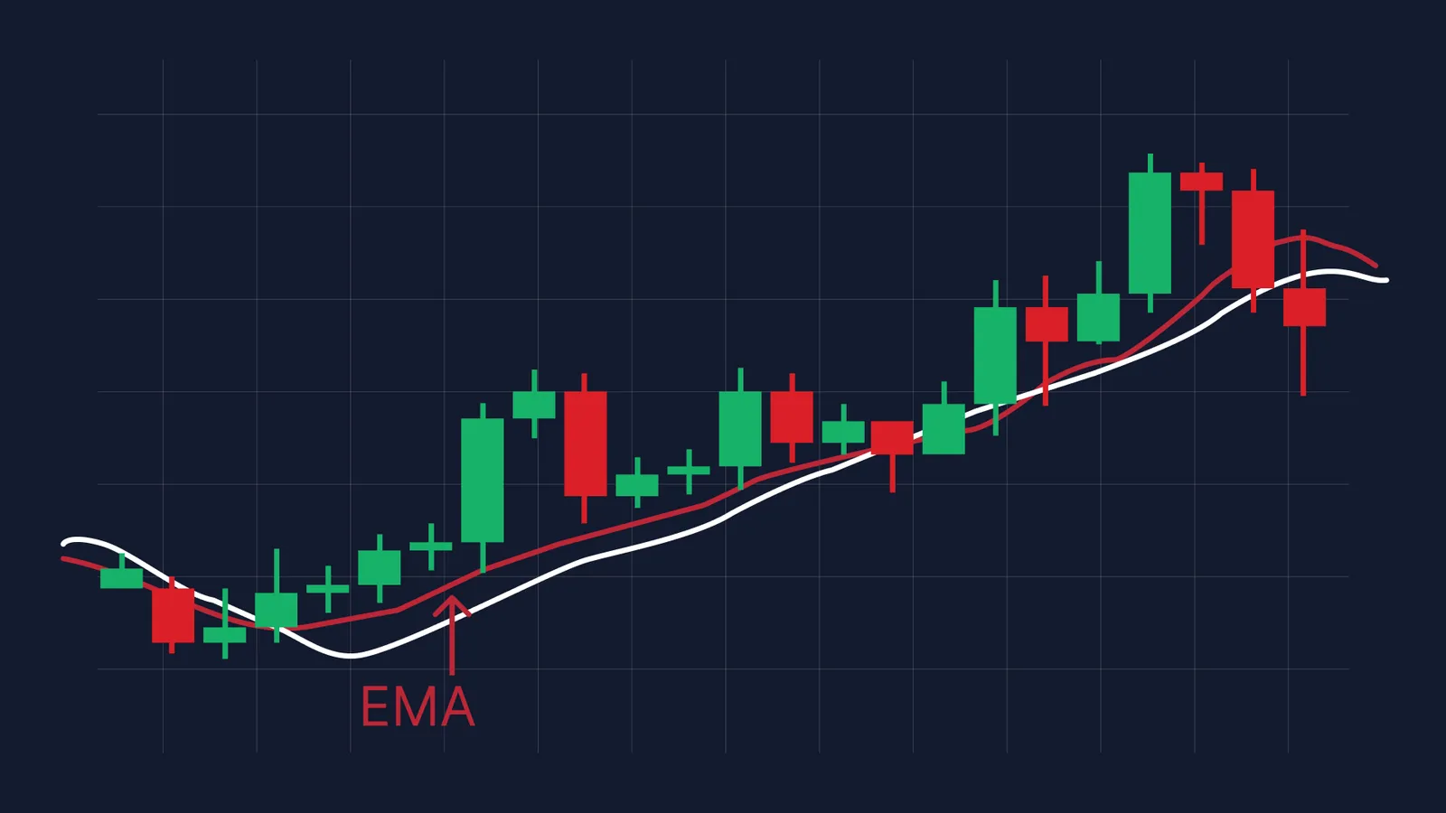
A familiar use of EMA in financial trading. My application used a running baseline to identify anomalous battery telemetry readings. Image source: Equiti.
EMA gave recent readings more influence while keeping only a compact running baseline per sensor:
ema_t = alpha * x_t + (1 - alpha) * ema_previous
Here, x_t is the incoming reading and alpha is a smoothing factor between 0 and 1. A larger alpha adapts faster; a smaller one produces a steadier baseline. Older readings receive exponentially decreasing weight, as described in NIST's explanation of exponential smoothing.
The distinction is between the baseline and the anomaly decision. EMA alone does not flag a spike: the detector evaluates how far a reading departs from the baseline. Conceptually, that departure can be expressed as:
deviation_t = abs(x_t - ema_previous)
This illustrates comparison with the baseline before incorporating the new reading; it is not a reconstruction of the production threshold rule. The important design choice was to use recent behavior to identify timestamps worth retaining, rather than relying only on the points selected for a chart.
EMA was a good fit for that goal because it adapted as a sensor's operating level changed without storing its full history. The tradeoff was responsiveness: a baseline that adapts too quickly can follow an anomaly, while one that adapts too slowly can lag behind a legitimate change in operation.
Cloud Fault Detection System
Impact: The fault detection feature was deployed to production, automatically generating fault events from live telemetry and surfacing them through dashboard alerts and AWS SES email notifications.
I contributed to the system's implementation across telemetry processing, fault retrieval, and notifications. The system consumed live measurements from AWS IoT Core MQTT topics and evaluated them against configurable thresholds retrieved from backend services.
My implementation work included:
- Building NestJS monitoring services to consume MQTT telemetry and evaluate threshold-based fault conditions.
- Caching threshold configurations to reduce repeated database lookups during telemetry processing.
- Implementing Athena-backed fault retrieval APIs and supporting historical investigation through Parquet-based data warehousing.
- Integrating fault detection with frontend dashboard alerts and email notifications through AWS SES.
Sensor Hysteresis and Fault Recovery
I also worked on hysteresis for transitions between fault severity levels. A sensor reading could move from normal to a high warning and then to a more severe high fault. Recovery needed to account for the current state: clearing the more severe fault did not necessarily mean the reading had returned to normal.
Separate trigger and recovery thresholds controlled these transitions. For example, a reading could trigger the more severe high fault above its upper threshold, then clear that state only after falling below its recovery threshold. If the high-warning condition still applied, the sensor would step back down to a warning rather than immediately returning to normal.
Separate activation and recovery thresholds prevented small sensor fluctuations from repeatedly triggering and clearing faults, while ensuring recovery followed the appropriate severity transitions.
Together, these components connected live fault detection with notifications and historical fault retrieval, giving users a way to investigate detected conditions after an alert.
Additional Contributions
Alongside these projects, I contributed to three areas of the platform:
- Operational tooling: React and MUI interfaces for deployment and monitoring, multi-step provisioning and firmware management tools, and AWS IoT Core job template integration.
- Reusable interfaces: Shared chart, table, and form components, plus dynamic filtering and search across dashboard tables.
- Backend and platform maintenance: NestJS API endpoints and business logic, role-based access control and user management features, bug fixes, testing, and code reviews.
Reflection
This work taught me to evaluate performance and information loss together. Moving calculations into SQL and reducing chart payloads made telemetry faster to explore, but a useful dashboard also needed to retain evidence of short-lived anomalies. Comparing cumulative statistics with EMA helped me connect an algorithm's treatment of history to a product requirement: showing the moments that matter, even across longer time ranges.